![]()
![]()
Implements conditional inference on normal variates as described in Lee, Sun, Sun and Taylor, “Exact Post Selection Inference, with Application to the Lasso.”
– Steven E. Pav, shabbychef@gmail.com
This package may be installed from CRAN; the latest version may be found on github via devtools, or installed via drat:
# CRAN
install.packages(c("epsiwal"))
# devtools
if (require(devtools)) {
    # latest greatest
    install_github("shabbychef/epsiwal")
}
# via drat:
if (require(drat)) {
    drat:::add("shabbychef")
    install.packages("epsiwal")
}First we perform some simulations under the null to show that the p-values are uniform. We draw a normal vector with identity covariance and zero mean, then flip the sign of each element to make them positive. We then perform inference on the sum of the mean values.
library(epsiwal)
p <- 20
mu <- rep(0, p)
Sigma <- diag(p)
A <- -diag(p)
b <- rep(0, p)
eta <- rep(1, p)
Sigma_eta <- diag(Sigma)
eta_mu <- as.numeric(t(eta) %*% mu)
set.seed(1234)
pvals <- replicate(1000, {
    y <- rnorm(p, mean = mu, sd = sqrt(diag(Sigma)))
    ay <- abs(y)
    pconnorm(y = ay, A = A, b = b, eta = eta, Sigma_eta = Sigma_eta,
        eta_mu = eta_mu)
})
qqplot(pvals, qunif(ppoints(length(pvals))), main = "p-values under procedure",
    ylab = "theoretical", xlab = "empirical")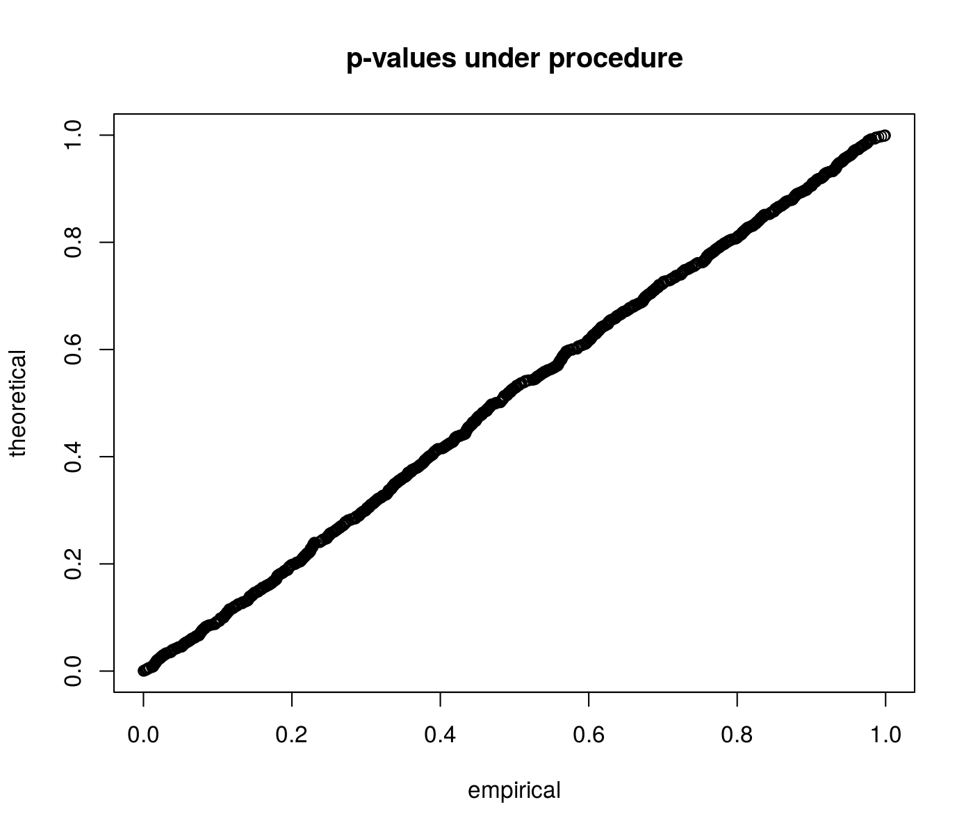
plot of chunk under_null_pvals
library(epsiwal)
p <- 20
mu <- rep(0, p)
Sigma <- diag(p)
A <- -diag(p)
b <- rep(0, p)
eta <- rep(1, p)
Sigma_eta <- diag(Sigma)
eta_mu <- as.numeric(t(eta) %*% mu)
type_I <- 0.05
set.seed(1234)
civals <- replicate(5000, {
    y <- rnorm(p, mean = mu, sd = sqrt(diag(Sigma)))
    ay <- abs(y)
    ci <- ci_connorm(y = ay, A = A, b = b, p = type_I,
        eta = eta, Sigma_eta = Sigma_eta)
})
cat("Empirical coverage of the", type_I, "confidence bound is around",
    mean(civals < eta_mu), ".\n")
## Empirical coverage of the 0.05 confidence bound is around 0.052 .The package supports the “Selective MLE” procedure of Reid, Taylor
and Tibshirani. This is via the mle_connorm function, or
the associated mle_connorm_max.
library(epsiwal)
p <- 20
mu <- rep(0, p)
Sigma <- diag(p)
A <- -diag(p)
b <- rep(0, p)
eta <- rep(1, p)
Sigma_eta <- diag(Sigma)
set.seed(1234)
y <- rnorm(p, mean = mu, sd = sqrt(diag(Sigma)))
ay <- abs(y)
mval <- mle_connorm(y = ay, A = A, b = b, eta = eta,
    Sigma_eta = Sigma_eta)
cat("MLE is ", mval, " while true value is 0.\n")
## MLE is 2.1 while true value is 0.A common problem is to perform inference on the maximum of a normal vector. This package provides convenience functions for this case when the vector is assumed to have a common variance and common correlation (equicorrelation).
Suppose we observe \(y_i \sim N(\mu_i, \sigma^2)\) with \(\mathrm{corr}(y_i, y_j) = \rho\). We find the maximum element \(y_k\) and want to perform inference on its mean \(\mu_k\), conditional on it being the maximum.
library(epsiwal)
set.seed(123)
n <- 8
sigma <- 1.2
rho <- 0.3
mu <- rnorm(n, mean = 2)

# Generate data
Sigma <- sigma^2 * ((1 - rho) * diag(n) + rho * matrix(1,
    n, n))
y <- MASS::mvrnorm(1, mu, Sigma)

# Find the maximum
k <- which.max(y)
yk <- y[k]
yk1 <- y[-k]

# what is the true value?
cat("True mu_k is:", mu[k], "\n")
## True mu_k is: 3.7# Inference on mu_k 1. P-value for a specific
# mu_k
p_val <- pconnorm_max(yk, yk1, mu_k = mu[k], sigma = sigma,
rho = rho)
cat("P-value for true mu_k:", p_val, "\n")## P-value for true mu_k: 0.94# 2. Confidence interval for mu_k
ci <- ci_connorm_max(yk, yk1, sigma = sigma, rho = rho)
cat("95% CI for mu_k:", ci, "\n")## 95% CI for mu_k: 8.3 3# 3. Maximum Likelihood Estimate for mu_k
mle <- mle_connorm_max(yk, yk1, sigma = sigma, rho = rho)
cat("MLE for mu_k:", mle, "\n")## MLE for mu_k: 5.8PSAT
package, which supports similar procedures, but is not yet on
CRAN.SelectiveInference
package, which implements similar inferential procedures under
quadratic constraints, as detailed in Tibshirani, R. J., Taylor, J.,
Lockhart, R. and Tibshirani, R. Exact Post-Selection Inference
for Sequential Regression Procedures.