![]()
![]()
MultiVariate (Dynamic) Generalized Additive Models
![]()
![]()
![]()
![]()
The mvgam 📦 fits Bayesian Dynamic Generalized Additive
Models (DGAMs) that can include highly flexible nonlinear predictor
effects, latent variables and multivariate time series models. The
package does this by relying on functionalities from the impressive
brms and
mgcv packages. Parameters are estimated
using the probabilistic programming language Stan, giving users access
to the most advanced Bayesian inference algorithms available. This
allows mvgam to fit a very wide range of models,
including:
You can install the stable package version from CRAN
using: install.packages('mvgam'), or install the latest
development version using:
devtools::install_github("nicholasjclark/mvgam"). You will
also need a working version of Stan installed (along with
either rstan and/or cmdstanr). Please refer to
installation links for Stan with rstan
here, or for Stan with
cmdstandr
here.

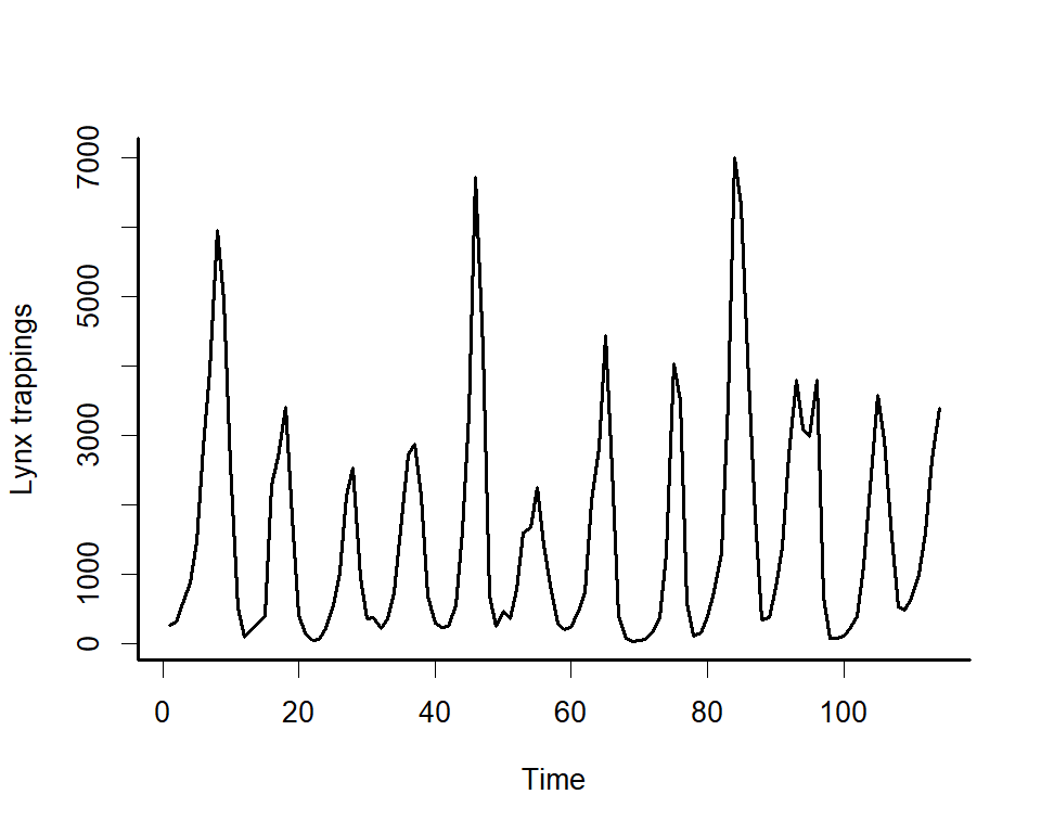
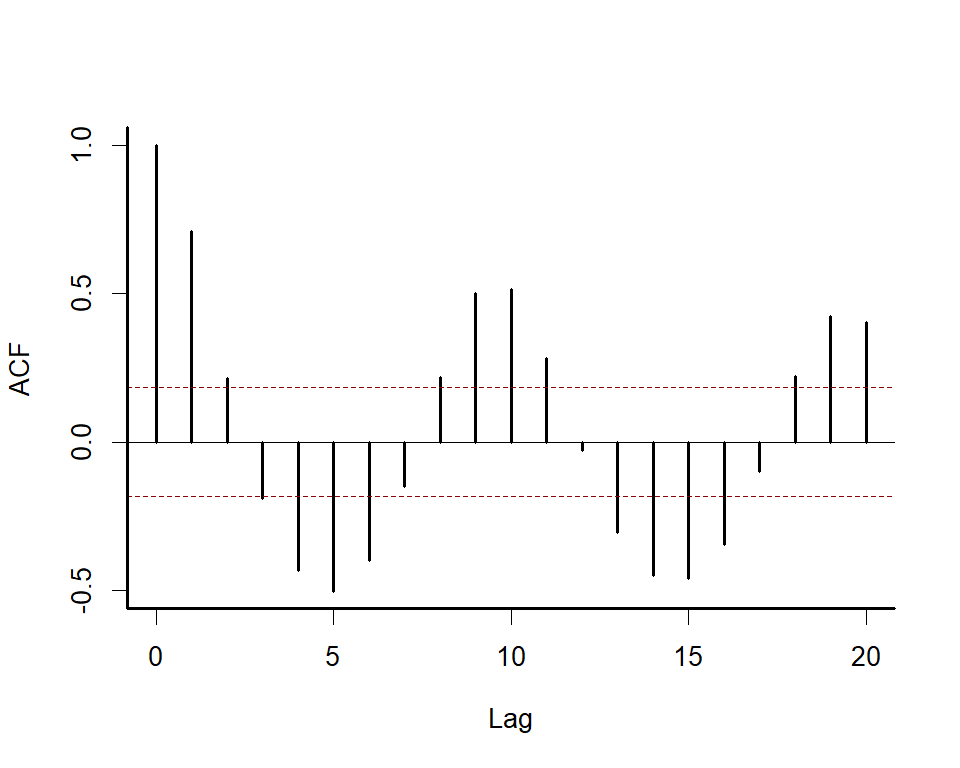
We can explore the package’s primary functions using one of it’s
built-in datasets. Use plot_mvgam_series() to inspect
features for time series from
the Portal
Project, which represent counts of baited captures for four desert
rodent species over time (see ?portal_data for more details
about the dataset).
data(portal_data)
plot_mvgam_series(
  data = portal_data,
  y = 'captures',
  series = 'all'
)
plot_mvgam_series(
  data = portal_data,
  y = 'captures',
  series = 1
)
plot_mvgam_series(
  data = portal_data,
  y = 'captures',
  series = 4
)
These plots show that the time series are count responses, with
missing data, many zeroes, seasonality and temporal autocorrelation all
present. These features make time series analysis and forecasting very
difficult using conventional software. But mvgam shines in
these tasks.
For most forecasting exercises, we’ll want to split the data into training and testing folds:
data_train <- portal_data %>%
  dplyr::filter(time <= 60)
data_test <- portal_data %>%
  dplyr::filter(time > 60 &
                  time <= 65)
Formulate an mvgam model; this model fits a State-Space
GAM in which each species has its own intercept, linear association with
ndvi_ma12 and potentially nonlinear association with
mintemp. These effects are estimated jointly with a full
time series model for the temporal dynamics (in this case a Vector
Autoregressive process). We assume the outcome follows a Poisson
distribution and will condition the model in Stan using
MCMC sampling with Cmdstan:
mod <- mvgam(
  # Observation model is empty as we don't have any
  # covariates that impact observation error
  formula = captures ~ 0,

  # Process model contains varying intercepts,
  # varying slopes of ndvi_ma12 and varying smooths
  # of mintemp for each series.
  # Temporal dynamics are modelled with a Vector
  # Autoregression (VAR(1))
  trend_formula = ~
    trend +
    s(trend, bs = 're', by = ndvi_ma12) +
    s(mintemp, bs = 'bs', by = trend) - 1,
  trend_model = VAR(cor = TRUE),

  # Obvservations are conditionally Poisson
  family = poisson(),

  # Condition on the training data
  data = data_train,
  backend = 'cmdstanr'
)
Using print() returns a quick summary of the object:
mod
#> GAM observation formula:
#> captures ~ 1
#>
#> GAM process formula:
#> ~trend + s(trend, bs = "re", by = ndvi_ma12) + s(mintemp, bs = "bs",
#> by = trend) - 1
#>
#> Family:
#> poisson
#>
#> Link function:
#> log
#>
#> Trend model:
#> VAR(cor = TRUE)
#>
#>
#> N latent factors:
#> 4
#>
#> N series:
#> 4
#>
#> N timepoints:
#> 60
#>
#> Status:
#> Fitted using Stan
#> 4 chains, each with iter = 2000; warmup = 1500; thin = 1
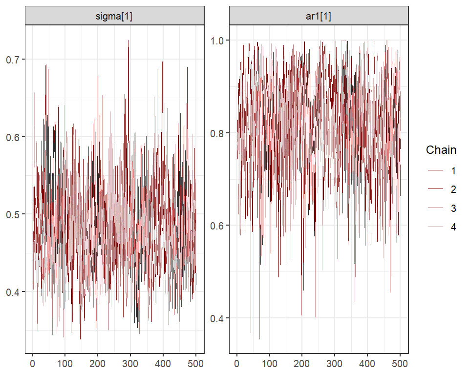
#> Total post-warmup draws = 2000Split Rhat and Effective Sample Size diagnostics show good convergence of model estimates
mcmc_plot(mod,
          type = 'rhat_hist')
#> `stat_bin()` using `bins = 30`. Pick better value `binwidth`.
mcmc_plot(mod,
          type = 'neff_hist')
#> `stat_bin()` using `bins = 30`. Pick better value `binwidth`.
Use conditional_effects() for a quick visualisation of
the main terms in model formulae
conditional_effects(mod,
                    type = 'link')


If you have the gratia package installed, it can also be
used to plot partial effects of smooths
require(gratia)
draw(mod,
     trend_effects = TRUE)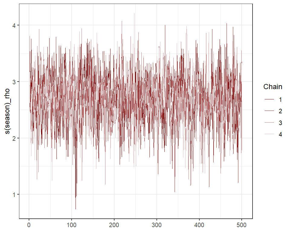
Or design more targeted plots using plot_predictions()
from the marginaleffects package
plot_predictions(
  mod,
  condition = c('ndvi_ma12',
                'series',
                'series'),
  type = 'link'
)
plot_predictions(
  mod,
  condition = c('mintemp',
                'series',
                'series'),
  type = 'link'
)
We can also view the model’s posterior predictions for the entire
series (testing and training). Forecasts can be scored using a range of
proper scoring rules. See ?score.mvgam_forecast for more
details
fcs <- forecast(mod,
                newdata = data_test)
plot(fcs, series = 1) +
  plot(fcs, series = 2) +
  plot(fcs, series = 3) +
  plot(fcs, series = 4)
#> Out of sample DRPS:
#> 8.23058125
#> Out of sample DRPS:
#> 5.33980075
#> Out of sample DRPS:
#> 8.71284175
#> Out of sample DRPS:
#> 3.83530975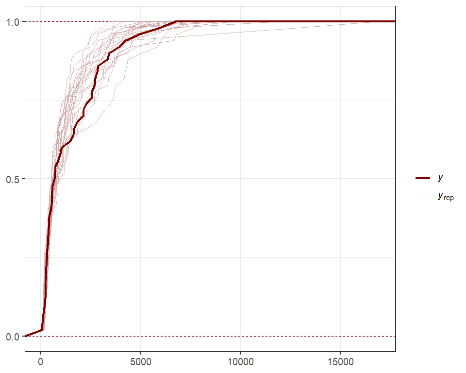
For Vector Autoregressions fit in mvgam, we can inspect
impulse response functions and forecast error variance
decompositions. The irf() function runs an Impulse
Response Function (IRF) simulation whereby a positive “shock” is
generated for a target process at time t = 0. All else
remaining stable, it then monitors how each of the remaining processes
in the latent VAR would be expected to respond over the forecast horizon
h. The function computes impulse responses for all
processes in the object and returns them in an array that can be plotted
using the S3 plot() function. Here we will use the
generalized IRF, which makes no assumptions about the order in which the
series appear in the VAR process, and inspect how each process is
expected to respond to a sudden, positive pulse from the other processes
over a horizon of 12 timepoints.
irfs <- irf(mod,
            h = 12,
            orthogonal = FALSE)
plot(irfs,
     series = 1)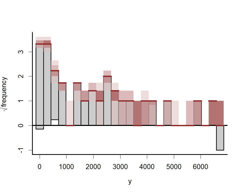
plot(irfs,
     series = 3)
Using the same logic as above, we can inspect forecast error variance
decompositions (FEVDs) for each process usingfevd(). This
type of analysis asks how orthogonal shocks to all process in the system
contribute to the variance of forecast uncertainty for a focal process
over increasing horizons. In other words, the proportion of the forecast
variance of each latent time series can be attributed to the effects of
the other series in the VAR process. FEVDs are useful because some
shocks may not be expected to cause variations in the short-term but may
cause longer-term fluctuations
fevds <- fevd(mod,
              h = 12)
plot(fevds)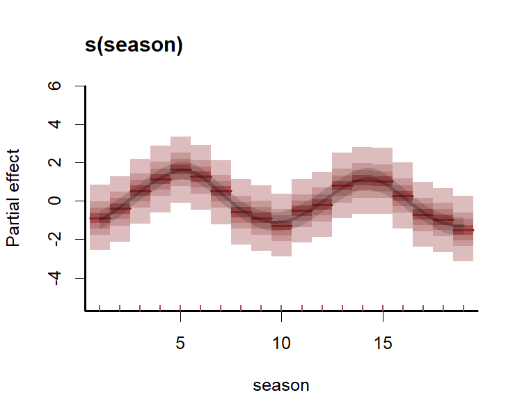
This plot shows that the variance of forecast uncertainty for each process is initially dominated by contributions from that same process (i.e. self-dependent effects) but that effects from other processes become more important over increasing forecast horizons. Given what we saw from the IRF plots above, these long-term contributions from interactions among the processes makes sense.
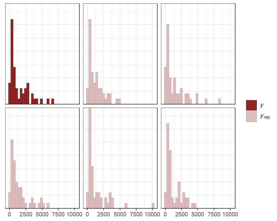
Plotting randomized quantile residuals over time for
each series can give useful information about what might be missing from
the model. We can use the highly versatile pp_check()
function to plot these:
pp_check(
  mod,
  type = 'resid_ribbon_grouped',
  group = 'series',
  x = 'time',
  ndraws = 200
)
When describing the model, it can be helpful to use the
how_to_cite() function to generate a scaffold for
describing the model and sampling details in scientific
communications
description <- how_to_cite(mod)

description

#> Methods text skeleton
#> We used the R package mvgam (version 1.1.594; Clark & Wells, 2023) to
#>   construct, fit and interrogate the model. mvgam fits Bayesian
#>   State-Space models that can include flexible predictor effects in both
#>   the process and observation components by incorporating functionalities
#>   from the brms (Burkner 2017), mgcv (Wood 2017) and splines2 (Wang & Yan,
#>   2023) packages. To encourage stability and prevent forecast variance
#>   from increasing indefinitely, we enforced stationarity of the Vector
#>   Autoregressive process following methods described by Heaps (2023) and
#>   Clark et al. (2025). The mvgam-constructed model and observed data were
#>   passed to the probabilistic programming environment Stan (version
#>   2.38.0; Carpenter et al. 2017, Stan Development Team 2026), specifically
#>   through the cmdstanr interface (Gabry & Cesnovar, 2021). We ran 4
#>   Hamiltonian Monte Carlo chains for 1500 warmup iterations and 500
#>   sampling iterations for joint posterior estimation. Rank normalized
#>   split Rhat (Vehtari et al. 2021) and effective sample sizes were used to
#>   monitor convergence.

#>
#> Primary references
#> Clark, NJ and Wells K (2023). Dynamic Generalized Additive Models
#>   (DGAMs) for forecasting discrete ecological time series. Methods in
#>   Ecology and Evolution, 14, 771-784. doi.org/10.1111/2041-210X.13974
#> Burkner, PC (2017). brms: An R Package for Bayesian Multilevel Models
#>   Using Stan. Journal of Statistical Software, 80(1), 1-28.
#>   doi:10.18637/jss.v080.i01
#> Wood, SN (2017). Generalized Additive Models: An Introduction with R
#>   (2nd edition). Chapman and Hall/CRC.
#> Wang W and Yan J (2021). Shape-Restricted Regression Splines with R
#>   Package splines2. Journal of Data Science, 19(3), 498-517.
#>   doi:10.6339/21-JDS1020 https://doi.org/10.6339/21-JDS1020.
#> Heaps, SE (2023). Enforcing stationarity through the prior in vector
#>   autoregressions. Journal of Computational and Graphical Statistics 32,
#>   74-83.
#> Clark NJ, Ernest SKM, Senyondo H, Simonis J, White EP, Yenni GM,
#>   Karunarathna KANK (2025). Beyond single-species models: leveraging
#>   multispecies forecasts to navigate the dynamics of ecological
#>   predictability. PeerJ 13:e18929.
#> Carpenter B, Gelman A, Hoffman MD, Lee D, Goodrich B, Betancourt M,
#>   Brubaker M, Guo J, Li P and Riddell A (2017). Stan: A probabilistic
#>   programming language. Journal of Statistical Software 76.
#> Gabry J, Cesnovar R, Johnson A, and Bronder S (2026). cmdstanr: R
#>   Interface to 'CmdStan'. https://mc-stan.org/cmdstanr/,
#>   https://discourse.mc-stan.org.
#> Vehtari A, Gelman A, Simpson D, Carpenter B, and Burkner P (2021).
#>   Rank-normalization, folding, and localization: An improved Rhat for
#>   assessing convergence of MCMC (with discussion). Bayesian Analysis 16(2)
#>   667-718. https://doi.org/10.1214/20-BA1221.
#>
#> Other useful references
#> Arel-Bundock V, Greifer N, and Heiss A (2024). How to interpret
#>   statistical models using marginaleffects for R and Python. Journal of
#>   Statistical Software, 111(9), 1-32.
#>   https://doi.org/10.18637/jss.v111.i09
#> Gabry J, Simpson D, Vehtari A, Betancourt M, and Gelman A (2019).
#>   Visualization in Bayesian workflow. Journal of the Royal Statatistical
#>   Society A, 182, 389-402. doi:10.1111/rssa.12378.
#> Vehtari A, Gelman A, and Gabry J (2017). Practical Bayesian model
#>   evaluation using leave-one-out cross-validation and WAIC. Statistics and
#>   Computing, 27, 1413-1432. doi:10.1007/s11222-016-9696-4.
#> Burkner PC, Gabry J, and Vehtari A. (2020). Approximate leave-future-out
#>   cross-validation for Bayesian time series models. Journal of Statistical
#>   Computation and Simulation, 90(14), 2499-2523.
#>   https://doi.org/10.1080/00949655.2020.1783262
The post-processing methods we have shown above are just the tip of
the iceberg. For a full list of methods to apply on fitted model
objects, type methods(class = "mvgam").
mvgam was originally designed to analyse and forecast
non-negative integer-valued data. But further development of
mvgam has resulted in support for a growing number of
observation families. Currently, the package can handle data for the
following:
gaussian() for real-valued datastudent_t() for heavy-tailed real-valued datalognormal() for non-negative real-valued dataGamma() for non-negative real-valued databetar() for proportional data on
(0,1)bernoulli() for binary datapoisson() for count datanb() for overdispersed count databinomial() for count data with known number of
trialsbeta_binomial() for overdispersed count data with known
number of trialsnmix() for count data with imperfect detection (unknown
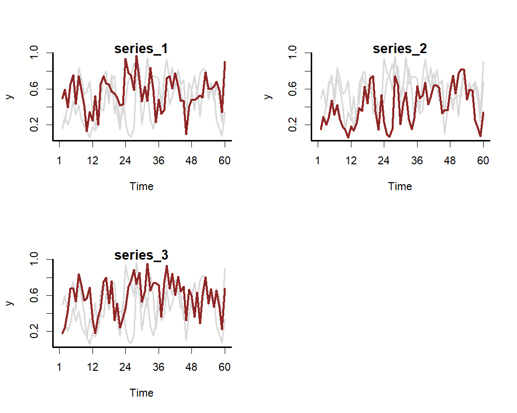
number of trials)See ??mvgam_families for more information. Below is a
simple example for simulating and modelling proportional data with
Beta observations over a set of seasonal series with
independent Gaussian Process dynamic trends:
set.seed(100)
data <- sim_mvgam(
  family = betar(),
  T = 80,
  trend_model = GP(),
  prop_trend = 0.5,
  seasonality = "shared"
)
plot_mvgam_series(
  data = data$data_train,
  series = "all"
)
mod <- mvgam(
y ~ s(season, bs = "cc", k = 7) +
s(season, by = series, m = 1, k = 5),
trend_model = GP(),
data = data$data_train,
newdata = data$data_test,
family = betar()
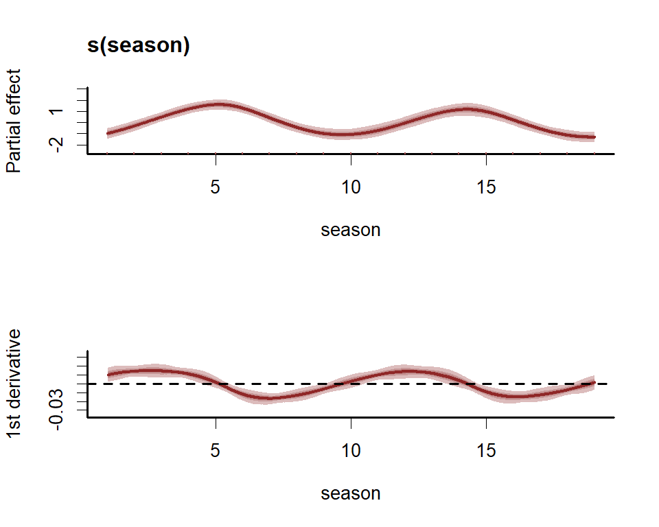
)Inspect the summary to see that the posterior now also contains
estimates for the Beta precision parameters ϕ.
summary(mod,
include_betas = FALSE)
#> GAM formula:
#> y ~ s(season, bs = "cc", k = 7) + s(season, by = series, m = 1,
#> k = 5)
#>
#> Family:
#> beta
#>
#> Link function:
#> logit
#>
#> Trend model:
#> GP()
#>
#> N series:
#> 3
#>
#> N timepoints:
#> 80
#>
#> Status:
#> Fitted using Stan
#> 4 chains, each with iter = 1000; warmup = 500; thin = 1
#> Total post-warmup draws = 2000
#>
#> Observation precision parameter estimates:
#> 2.5% 50% 97.5% Rhat n_eff
#> phi[1] 7.8 12.0 18.0 1 1829
#> phi[2] 5.6 8.6 13.0 1 1023
#> phi[3] 4.1 6.0 8.7 1 1404
#>
#> GAM coefficient (beta) estimates:
#> 2.5% 50% 97.5% Rhat n_eff
#> (Intercept) 0.11 0.45 0.7 1.01 602
#>
#> Approximate significance of GAM smooths:
#> edf Ref.df Chi.sq p-value
#> s(season) 3.9071 5 9.792 0.0653 .
#> s(season):seriesseries_1 1.0934 4 11.307 0.2695
#> s(season):seriesseries_2 2.5629 4 2.227 0.4544
#> s(season):seriesseries_3 0.8565 4 6.556 0.5358
#> ---
#> Signif. codes: 0 '***' 0.001 '**' 0.01 '*' 0.05 '.' 0.1 ' ' 1
#>
#> marginal deviation:
#> 2.5% 50% 97.5% Rhat n_eff
#> alpha_gp[1] 0.150 0.40 0.88 1.00 828
#> alpha_gp[2] 0.570 0.93 1.50 1.00 1018
#> alpha_gp[3] 0.052 0.40 0.92 1.01 672
#>
#> length scale:
#> 2.5% 50% 97.5% Rhat n_eff
#> rho_gp[1] 1.2 3.6 11 1.00 1482
#> rho_gp[2] 3.0 12.0 30 1.01 367
#> rho_gp[3] 1.3 4.9 26 1.00 532
#>
#> Stan MCMC diagnostics:
#> ✔ No issues with effective samples per iteration
#> ✔ Rhat looks good for all parameters
#> ✔ No issues with divergences
#> ✔ No issues with maximum tree depth
#>
#> Samples were drawn using sampling(hmc). For each parameter, n_eff is a
#> crude measure of effective sample size, and Rhat is the potential scale
#> reduction factor on split MCMC chains (at convergence, Rhat = 1)
#>
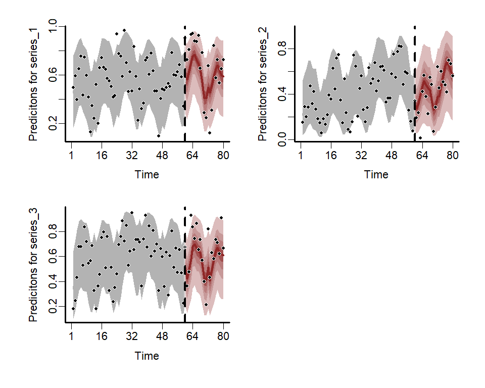
#> Use how_to_cite() to get started describing this modelPlot the hindcast and forecast distributions for each series
library(patchwork)
fc <- forecast(mod)
wrap_plots(
  plot(fc, series = 1),
  plot(fc, series = 2),
  plot(fc, series = 3),
  ncol = 2
)
There are many more extended uses of mvgam, including
the ability to fit hierarchical State-Space GAMs that include dynamic
and spatially varying coefficient models, dynamic factors, Joint Species
Distribution Models and much more. See the
package documentation for more details.
mvgam can also be used to generate all necessary data
structures and modelling code necessary to fit DGAMs using
Stan. This can be helpful if users wish to make changes to
the model to better suit their own bespoke research / analysis goals.
The Stan Discourse is a helpful place to
troubleshoot.
mvgam and
related softwareWhen using any software please make sure to appropriately acknowledge the hard work that developers and maintainers put into making these packages available. Citations are currently the best way to formally acknowledge this work (but feel free to ⭐ this repo as well).
When using mvgam, please cite the following:
Clark, N.J. and Wells, K. (2023). Dynamic Generalized Additive Models (DGAMs) for forecasting discrete ecological time series. Methods in Ecology and Evolution. DOI: https://doi.org/10.1111/2041-210X.13974
As mvgam acts as an interface to Stan,
please additionally cite:
Carpenter B., Gelman A., Hoffman M. D., Lee D., Goodrich B., Betancourt M., Brubaker M., Guo J., Li P., and Riddell A. (2017). Stan: A probabilistic programming language. Journal of Statistical Software. 76(1). DOI: https://doi.org/10.18637/jss.v076.i01
mvgam relies on several other R packages
and, of course, on R itself. Use how_to_cite()
to simplify the process of finding appropriate citations for your
software setup.
If you encounter a clear bug, please file an issue with a minimal
reproducible example on GitHub. Please
also feel free to use the mvgam
Discussion Board to hunt for or post other discussion topics related
to the package, and do check out the mvgam
Changelog for any updates about recent upgrades that the package has
incorporated.
A series of vignettes cover data formatting, forecasting and several extended case studies of DGAMs. A number of other examples, including some step-by-step introductory webinars, have also been compiled:
mvgam
packagemgcv and mvgammvgamI’m actively seeking PhD students and other researchers to work in
the areas of ecological forecasting, multivariate model evaluation and
development of mvgam. Please reach out if you are
interested (n.clark’at’uq.edu.au). Other contributions are also very
welcome, but please see The
Contributor Instructions for general guidelines. Note that by
participating in this project you agree to abide by the terms of its Contributor Code of
Conduct.
The mvgam project is licensed under an MIT
open source license